D. Kelly O'Day, of the Process Trends web site, has a new
Charts & Graphs blog, and
his first post comments on the US Census Bureau's Current Population Reports data discussed by
Jorge Camoes, and
Andreas Lipphardt at xlcubed.com, as an example of a confusing data set with too much detail, or is it just detail in need of sensitive presentation?

(as reader michael rightly points out in comments on the XLCubed post, this can't be showing the rise of income disparity, because it's percentage of households against fixed income level, not percentage of income against fixed household quantiles. Also, the series tops out at $100k, which is peanuts compared to the super-rich levels where the income transfer of the last few decades has really been most spectacular.)
Kelly abandons the time series approach to present the two end points in a dot plot:

However, I think that reducing the curves to a pair of points, one in 1967 and one in 2007, loses a lot of information that the full time series has to tell. So, in the spirit of defending loss aversion, I wondered if a readable time series graph could be constructed that would give real insights into the census table.
First, I made it a cumulative graph, so each income bracket now goes from zero to n(i), not n(i-1) to n(i). This means the lines can't cross any more, which should help:

I eliminated the >$100k line, as this is now by definition 100% of the households, cumulatively. As we see, the percentage of households making under $100k in constant dollars falls steadily from 1967 to 2005, which is just what we would expect from economic growth, and a desirable result. You want more people getting richer. However, this does not carry through to all income levels, which fall by less and less.
Perhaps this is an artifact of the linear scale, as written about by
Jon Peltier and
Nicolas Bissantz recently. So I tried it with a log scale instead:

(fully accepting Jon's comment that log scales do an equal injustice to the upper values, when the data is values equally distributed within an upper limit instead of proportionally distributed to infinity)
The surprising result is that the <$5k income level contains almost as many households in 2005 as in 1967, and significantly more than in the 70s, after a fall in the 60s. After a modest fall in the 90s, it rises again after 2000, as do all the other income levels below $100k. If we have said a fall is a good thing, then a rise must be bad. So the full time series data do contain a shocking insight, but it's to be found not at the upper levels but the lower ones, and not just by comparing 1967 to 2005, but following the trend down, then up. The dot plot can only tell a story of average improvement between 1967-2007, which masks a story of advance and retreat.


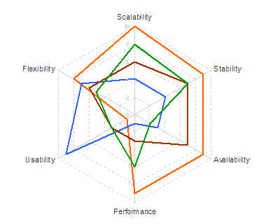 Not very informative. So he tries it as a "petal chart"
 Still not showing much. The circular formats of radar and petal charts don't really add value in this case, since we expect to be able to sort best from worst, and we don't really care if the best comes round to meet the worst, like the worm Ouroboros chomping on its own tail.
 So why not just show it as a table?
 I've re-ordered the criteria and options to show a rough diagonal trend. The criteria are obviously re-orderable categories, and I assume the options are, even though they're numbered 1-4. I take it that's just anonymising. Clearly Option 1 is the package for you if performance and scalability are what you're looking for, while you should consider option 2 if you really care about usability and flexibility. Sometimes the options in the middle excel at some crieria in the middle, but in this case options 3 and 4 don't really have anything to offer against the all-round competence of option 1.
 Finally, has re-ordering helped the spider?
 Sadly, no.


